Tumour in normal contamination (TINC), Part 1: How to avoid throwing the champagne out with the cork
By Olena Yavorska onOur approach to variant recovery when faced with a contaminated germline during tumour variant detection
An individual has on average one variant per 1000 base pairs, thus we expect their germline to have roughly 3-4 million variants. We are born with these variants, with most inherited from our parents in a Mendelian fashion (recall the Punnet squares drawn in school), although some will also be unique to us. As one might expect, many of these variants are common across a large population, and the majority of these common variants won’t pose any risks to people’s health in isolation.
The DNA in our cells slowly accumulates variants as we age, this is sometimes due to errors introduced during DNA replication, and sometimes due to exposure to environments that damage our DNA, e.g. carcinogens such as smoking or UV light. In some cases, when enough genes or regions regulating cell proliferation or apoptosis acquire variants, normal cell growth can be deregulated, and a tumour may begin to form. If our goal is to understand the development of the tumour, we need to identify mutations specific to the tumour cells. Recall that we already have 3-4 million variants that the individual was born with, and all these variants will also be present in the DNA of the tumour, i.e. normal genomic variation forms a significant haystack that the tumour-specific variant needles need to be detected in.
Let’s introduce an example. In Figure 1 we show a normal diploid region of DNA from a patient, with one copy of the maternal and one of the paternal chromosome. The germline contains some common variants as well as some that are rare. We focus on the paternal chromosome for simplicity and assume that some new tumour causing variants were acquired on that chromosome. Two of these are found in every tumour cell, so must have occurred early in the development of the tumour, whereas another is only present in 30% of cells. Upon sequencing a representative sample of the tumour, we would expect to see both the germline as well as the tumour-specific variants.
Note: We do not usually differentiate between paternal and maternal origin and calculate variant allele frequencies (VAFs) based on all the data available for a locus. In this case we expect 50% of the DNA to be maternal in origin since it’s a normal diploid region. Therefore, the acquired tumour variants can have a maximum VAF of 50% as they are heterozygous.
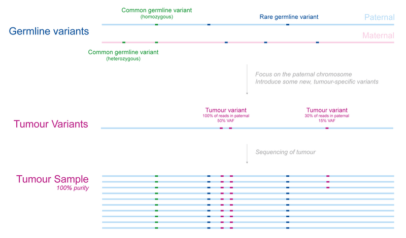
Figure 1
Tumour-normal subtraction with an uncontaminated germline
In cancer genomics, identification of new, potentially important tumour-specific mutations requires not only the DNA of the tumour sample, but also the germline. We can identify variants that are new by finding variants that are present in the tumour, but absent from the germline, this is usually called tumour-normal subtraction.
In Figure 2 we show how this approach works for our previously introduced patient. Using a high quality germline sample without any tumour cells, we can easily identify variants in the tumour that are absent from the germline. Importantly, this is even the case when the purity of the tumour sample isn’t 100%, as differentiating between cancerous and normal cells is often quite tricky.
Note: The VAFs are reported relative to the sample as opposed to the tumour. This is an important consideration when dealing with samples with low tumour purity as the calculated VAF will be purity x tumour VAF.
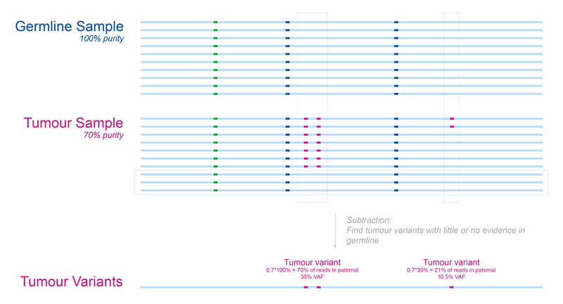
Figure 2
The problem with tumour in normal contamination (TINC)
Most algorithms expect that the germline is tumour-free or contains very few cells from the tumour. Unfortunately, it is not always possible to collect a germline sample that is completely free of cancer cells, particularly for patients with haematological cancers. In such cases, sufficiently high tumour in normal contamination (TINC) results in some tumour variants being mislabelled as germline during subtraction.
Suppose that the germline sample for our patient has 30% tumour cells as illustrated in Figure 3 (this is an extreme example). We run into a problem when performing the tumour-normal subtraction previously introduced: two of the tumour-specific variants are missing from the tumour variants group. In other words, if the TINC level is high enough, then tumour variants can be mislabelled as germline.
Note: It’s clear from this example why high-VAF variants are most affected by TINC since they are more likely to be present in a random sample of the contaminating cells.
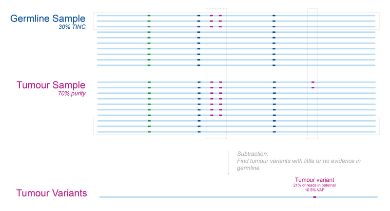
Figure 3
Ideally TINC would be avoided but extracting a pure germline sample from patients with haematological malignancies can prove difficult as the blood itself contains tumour cells. Until germline options which generally result in less TINC (such as skin biopsies and cultured fibroblasts) are adopted more widely, a computational method can help us prevent some of these tumour variants from being erroneously subtracted.
The TINC pipeline
At Genomics England, we take the possibility of TINC into consideration when analysing samples from individuals with haematological malignancies. We begin by estimating the contamination in the germline with the TINC package. If the germline is considered to be contaminated (>1% tumour DNA), then we use a germline from an unrelated individual of the same sex (unmatched germline) to help retrieve true somatic variants.
To illustrate this approach, let’s go back to our patient. In Figure 4 we can visualise what happens if we try tumour-normal subtraction when the germline comes from another individual. In this scenario, we identify all the tumour-specific as well as the patient’s germline variants.
Note: The specific unmatched germline used is less important than one might expect. Since the main aim of this step is to find as many actionable tumour-specific variants as possible, any germline with the same sex and without clear cancer predispositions should be sufficient.
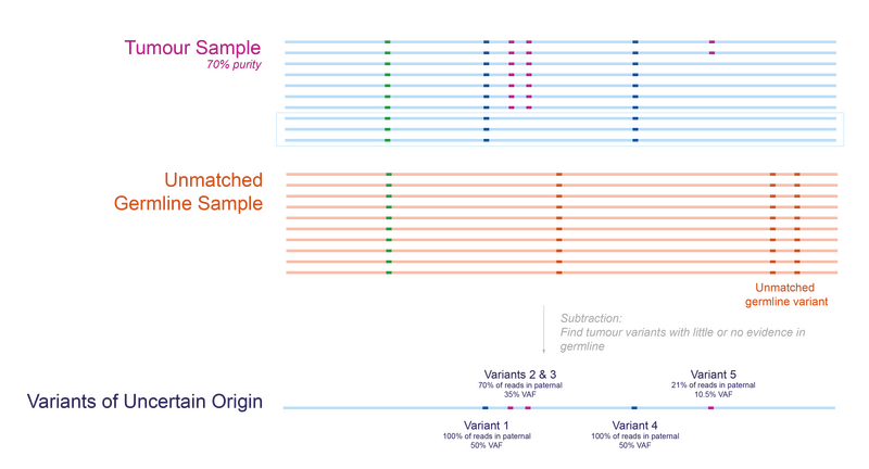
Figure 4
If we combine the results from the two analyses, tumour-normal subtraction and tumour-unmatched normal subtraction, we end up with two groups of variants of interest (Figure 5). We can be confident that the variants found in the analysis with matched germline sample are tumour-specific, we call this the somatic group. We cannot be certain whether variants detected only using the unmatched germline sample are tumour-specific or rare germline variants, so we call these ‘variants of uncertain origin’, but this analysis can identify clinically relevant variants in the tumour that would otherwise be missed.
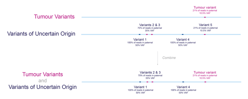
Figure 5
To help identify variants among the variants of uncertain origin that are likely to be germline variants, we filter out any variants that are commonly found in the population (with an allele frequency exceeding 1%). This ensures that most germline variants with a low probability of being pathogenic are removed.
Note: While we have used small variants in these examples, a similar approach works for structural variants. The main difference comes from the filtering step and how ‘un-interesting’ changes are defined. We will describe the downstream filtering approach in detail in Part 2.
To ensure that no actionable variants are missed, both the somatic and variants of uncertain origin are considered in the interpretation and prioritised for clinical review based on their proximity to clinically actionable regions (genes or regulatory regions). Thus, any variants of somatic or uncertain origin that are likely to be clinically actionable are highlighted and can be investigated further. A summary of the pipeline is shown in Figure 6 below.
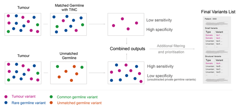
Figure 6
In a follow-up blog we will explain the downstream filtering in more detail, the results of the validation, and highlight some of the shortcomings of this approach – stay tuned!