Tumour in normal contamination (TINC) Part 2: Approaching variant recovery
By Olena Yavorska and Nadezda Volkova onIn Part 1 of this 2-part series, we broadly introduced our approach to tumour in normal contamination (TINC). In this instalment, we expand further on the details and limitations of our methodology.
If you aren’t familiar with the problem of TINC and unmatched normal sample subtraction, have a read of part 1 before continuing.
Filtering out common germline variants
Previously, we described a hybrid pipeline that uses both variant calling with an unmatched normal sample, and the traditional matched normal algorithm to recover variants missed due to tumour reads in the matched normal sample (Figure 1).
While unmatched normal subtraction is useful for increasing sensitivity of tumour variant detection, it causes a specificity drop because of the patient’s ‘rare’ germline variants, a.k.a those that didn’t overlap with any variants in the unmatched normal sample.
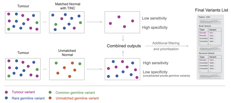
Figure 1
So how could we effectively filter out germline variants overloading the tumour variant calling results?
Naturally, we could take more unmatched normal samples and hope that some germline variants occur in these. We would then only select the overlap of multiple subtraction runs, with all the unmatched normal samples as our final tumour variant set.
While subtracting many normal samples is possible, this is a very inefficient approach computationally. If we consider a germline variant that occurs in just 1/100 healthy people to be common, we would need to perform variant calling another 100 times.
Fortunately, many healthy people’s genomes have been already sequenced, which allowed for the creation of several databases aggregating information about the population level occurrence of germline variants across healthy, unrelated individuals.
Filtering out common germline variants can result in lower sensitivity if we incorrectly classify a tumour-specific variant as germline. However, even if a common germline variant is tumour-specific for a particular patient, this variant is unlikely to be oncogenic and clinically actionable due to its high prevalence in normal tissues.
Population Allele Frequency
Variant Allele Fraction (VAF) vs Population Allele Frequency (AF) explained
Let us begin by interpreting what the population allele frequency of a variant represents. The variant allele fraction (VAF) is calculated as the proportion of reads that support the variant within a sample. The population allele frequency measures the proportion of alleles that show evidence of a given variant in a certain population of individuals.
In Figure 2, we illustrate the difference between the two metrics. We present 4 normal samples, each sequenced to a depth of 10, with some of their variants highlighted.
We first note the region shown is diploid, thus the total number of alleles to consider for these 4 samples is 8. To calculate population allele frequency, we need to genotype the samples, or determine the alleles each individual is carrying across the loci of interest.
In our example, we say that a variant is present on one allele if around 50% of reads in a sample show evidence of the variant. We say the variant is present in two alleles if over 70% of reads show evidence of the variant (this process is more sophisticated in practice).
Now we can calculate the population AF (bottom of Figure 2).
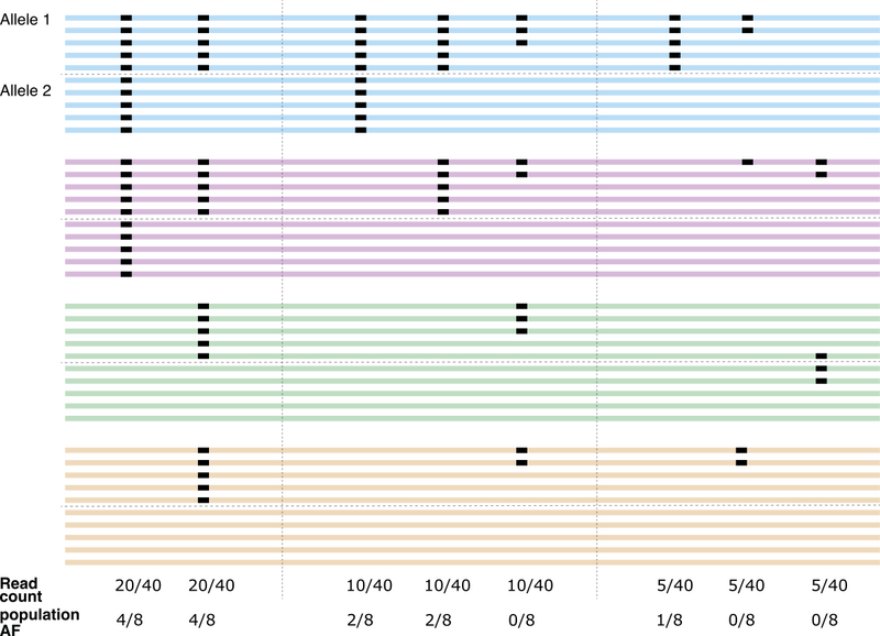
Figure 2
How to pick the population
The population itself is very important for interpretation. When constructing a set of individuals to use as our population dataset, we must carefully consider confounding factors and ensure suitability for our comparison.
Ideally, the set should serve as a representative sample from the general population. It should contain the same background factors as those impacting the sample or samples of interest in terms of ethnic diversity, disease status, and technical aspects (sample handling and sequencing). It is also important to ensure that the population we choose is large enough, as small sample sizes may lead to inaccurate estimates of true population allele frequencies.
We note here that the choice of thresholds used to define a ‘common’ variant is somewhat subjective – should a variant be considered rare if it’s only found in 1% of the population? 0.1% of the population? 0.000001% of the population? There is no correct answer here, but the majority of clinical laboratories across the world would use 1% as a cut-off (see reference here).
Panel of Normals for flagging sequencing artifacts
Apart from the germline variants, there is another source of false positive results in variant calling with unmatched normal (and sometimes even with a matched normal) - sequencing artifacts.
DNA preparation and sequencing are not perfect, and due to the nature of the sequencing-by-synthesis process we use, some errors are to be expected. These will normally be pronounced as mismatches occurring in one or just a few reads. We expect that most of these will be filtered out due to the normal variant subtraction during variant calling, as they would be likely to occur in both tumour and normal samples.
However, some such variants could still make their way through due to the difference in coverage, as tumour samples are normally sequenced to a greater depth (about 100x) than the normal samples (30x).
Remember those low VAF nucleotide changes observed across multiple individuals in Figure 2? Looking at those comes in handy when assessing whether low VAF mismatches in the tumour samples could be sequencing artifacts.
First, we build a list of read counts for alternative bases for all genomic positions across a large number of normal genomes (where no genuine low VAF variants are expected), called a noise panel of normals (noisePON).
This provides an expectation of an artifact at each position. We can then assess whether the proportion of reads supporting a particular nucleotide change in a tumour sample is higher than the expected one using Fisher Exact test.
Fisher Exact test (see reference here ) uses hypergeometric distribution to calculate the probability of seeing the alternative and reference base counts in a certain position we observed in the sample of interest. It considers the prior values we calculated from the noisePON. The lower this probability, the higher the chance there is a real variant in this position.
By transforming this probability into a quality score, we can highlight suspicious variants with low scores as common in our noisePON. We were able to find an optimal cut-off on this score that improved the variant calling precision on TRACERx lung cancer sample set up to 99% without any loss in sensitivity.
Filtering based on Population Frequencies at Genomics England
Small Variant Population AFs
At Genomics England, we use both internal and external databases to identify small germline variants that are common.
The samples in our internal dataset are representative of the population that we enrol, and thus should provide an accurate distribution for most individuals. The current internal cohort contains summarised population AFs across roughly 1,600 Genomics England patients.
In addition to the internal population AFs, we also use the population AFs from the Genome Aggregation Database (gnomAD v2.1.1). This database contains data aggregated from 15,708 whole genome sequencing samples across various ethnicities, and will provide better coverage for a more diverse group of people.
Our standard matched tumour-normal pipeline does not filter out common germline variants from the somatic calls. Instead, these are flagged whenever the AF exceeds 1% in either of the above populations.
In contrast, for variants that only come from unmatched analysis, any variants with AF exceeding 1% in either of the above populations are filtered out, while those with 0.1% < VAF < 1.0% are flagged as they likely represent rare germline variants.
We are currently in the process of benchmarking the expansion of these panels. The internal panels being tested include data across over 66,000 individuals. Similarly, transitioning to gnomAD v3.0 will mean better coverage across many new ethnicities. These updates will better highlight variants that are common in certain subgroups or are harder to detect due to genomic context.
Structural Variant Population AFs
To define a common structural variant (SV), let us start by recalling the basic types of structural variants (SVs) used in our variant calling procedure (Figure 3):
- Translocations (BND)
- Large insertions (INS) and deletions (DEL)
- Duplications (DUP)
- Inversions (INV)
In each case, the variant is defined based on the start and end coordinates (breakpoints, BPs), or the two break-end positions in the case of translocations.
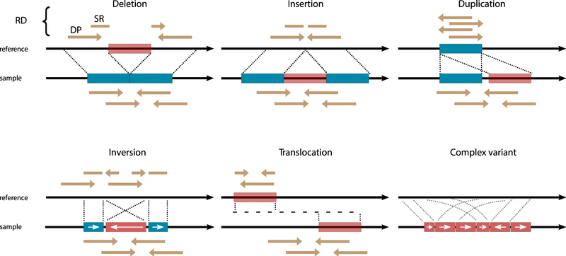
Figure 3. Schematic of each SV type (see reference here)
There is often some ambiguity regarding the exact location of the breakpoints, e.g., when the break resides within a simple repeat region, or a region with microhomology.
This ambiguity is represented by confidence intervals in the outputs from structural variant (SV) callers such that a small confidence interval indicates that the breakpoint is well defined.
During our investigations, we considered two major approaches:
- Unique SV panels for each variant type (BND, DEL, DUP, INS, INV)
- A breakpoint (BP) panel which combines the information across all SV types and focusses on the frequency of the breakpoints themselves
We discovered that the aggregated BP panel outperformed the SV panels in terms of increasing specificity when detecting structural variants using an unmatched normal sample. This was largely a consequence of the BP panel performing better in hard-to-map regions such as Alu repeats.
In Figure 4, we can see a well-defined breakpoint compared to ones with ambiguity. While the top panel shows very clear start and end coordinates of the region, the variation of deletion width in the bottom panel illustrates a variant in a more complex genomic landscape, where we can limit the true breakpoint to a region but not a single base.
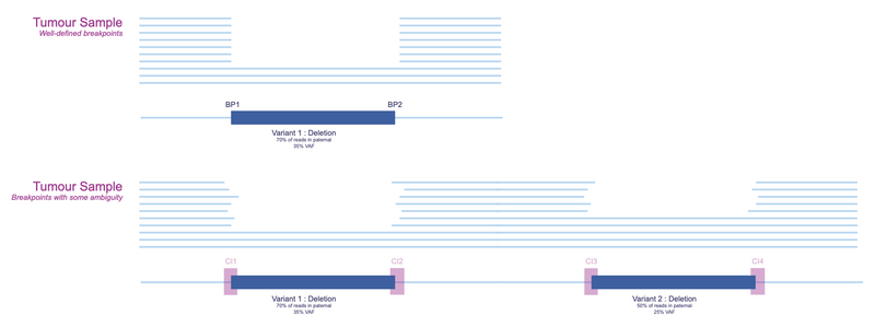
Figure 4. Example of confidence intervals
We created internal panels for structural variant filtering by taking these confidence intervals into consideration. Our aim for structural variants was to check whether the breakpoints of a variant were commonly found in a large population of normal samples.
In Figure 5, we present a stretch of DNA with confidence intervals of detected deletions highlighted for 10 normal samples.
The regions with high likelihood of a breakpoint are clearly visible. There are two regions where 50% of individuals have a detected deletion breakpoint. If we aggregate across a large population, we can draw a distribution showing the frequency of a deletion breakpoint at each base (and consequently each region bounded by some confidence interval).
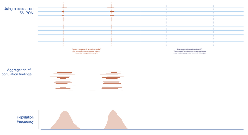
Figure 5. Creating the BP PON
In Figure 6, we return to our variants of interest and illustrate how the breakpoints can be assessed based on germline population frequencies. It is clear that the breakpoints of Variant 1 (left) are much more common in the population compared to those of Variant 2 (right). This would suggest that Variant 2 is more likely to be tumour specific.
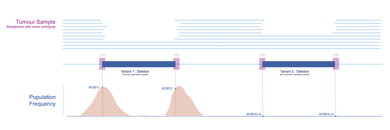
Figure 6. Using the PON
The resulting AFs can be interpreted as highlighting places in the genome which contain structural variant breakpoints that are either common across healthy individuals (but not included in the reference) or are particularly prone to artifacts.
Using two unique populations
Recall the importance of using a representative population to build the background distribution. During our preliminary investigations, we noticed that the distributions of SVs called by Manta differ depending on whether they’re called in a somatic-germline or germline-only mode.
We found systematically more SVs in the germline whenever the tumour sample was provided. Based on these findings, we decided to create two unique databases of common germline SVs as follows:
- We called SVs using germline-only mode across ~2,200 Covid patients. These individuals were otherwise healthy, meaning that any SVs with pre-dispositions to cancer shouldn’t show up at elevated frequencies.
- We called SVs in somatic-germline mode for ~2,700 cancer patients, focussing on the resulting germline SVs. This set would be most similar in terms of distributions of structural variants to the calls we would obtain from the matched and unmatched analyses.
These were the populations we utilised when we first introduced the panels of normal for SVs. By the end of 2023, we have many more SV calling datasets for both tumour-normal pairs and single normal samples, and will expand these datasets to better cater to the needs of incoming samples which are now exclusively sequenced with Illumina NovaSeq machines.
Similar to small variants, we flag somatic SVs where the maximum breakpoint AF exceeds 1% in either of the above distributions in matched tumour-normal analyses. Since there are multiple BPs per SV (start and end for deletions for example), we use the maximum of the frequencies to decide whether the variant should be flagged as common.
For SVs resulting from unmatched analyses, variants with breakpoints that exceed 1% AF in either cohort are filtered out. Those in the range between 0.1% and 1% are flagged as potential rare germline or artifact events.
Limitations
Filtering out common germline variant and sequencing artifacts is a crucial step in removing the false positive findings in our hybrid workflow.
The efficacy of filtering is largely defined by the quality of datasets: whether they are large and diverse enough. However, even with the best available databases, population frequency-based filtering may not be sufficient.
Our analysis shows that the specificity or the true negative rate of small variant detection in clinically relevant genes is still only about 25%. This means that 3 potentially germline variants are reported for each true somatic variant. The true negative rate for structural variants is a bit higher – about 40% – which still corresponds to 1-2 potentially germline SVs being reported for each true somatic SV (see reference here).
What can we do to further improve variant reporting for TINC cases?
There are other features that can hint as to whether a variant is somatic or germline, including VAF, the type of the variant and genomic location. Currently, all of these must be manually investigated for each variant of interest that was detected only in the unmatched normal variant calling.
Several machine learning-based classifiers have been developed in the past years to help distinguish between germline and somatic variants in tumour only variant calling outputs (find an example here or another example here).
We are currently investigating whether we could implement any of them at Genomics England to provide a confidence score for each variant. This would indicate whether it is more likely to be a somatic or germline variant, which should relieve the burden on the clinical scientists.
Want to read more?
Check out the other bioinformatics blogs on the Genomics England website.